Features Premiere
In the last section, we exposed you to the types of problems that are solvable with machine learning. We also mentioned that with enough good data, it's simply amazing what you can get a computer to do. Part of having good data is ensuring your data is organized so it can be processed. To be usable by SciKit-Learn, the machine learning library for Python you'll be using in this course, your data needs to be organized into matrix of samples and features:
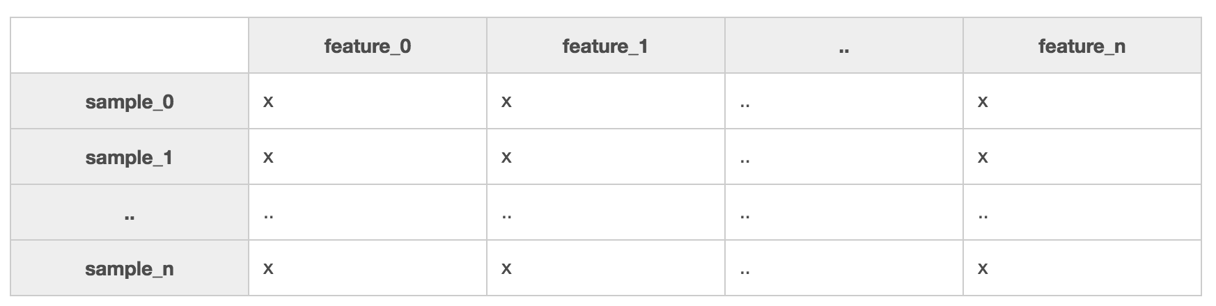
A sample is any phenomenon you can describe with quantitative traits. They are represented in your dataset by rows. If you were building a dataset of 'companies', each sample would be details about a company. When it's said that you need a lot of data, what is generally meant is that you need many samples.
Features are those quantitative traits that describe your samples. They might be numeric or textual, for example, CompanyName is a textual feature in your 'companies' dataset. Different samples might result in values such as 'Microsoft', 'EdX', or 'Coding Dojo' for the CompanyName feature. If CompanyRating were a numeric feature in the same dataset, its value might have score between 1 and 5 for each company:

Feature Types
There are many synonymous names for features. The background of the speaker, as well as the context of the conversation usually dictates which term is used:
Attribute - Features are a quantitative attributes of the samples being observed
Axis - Features are orthogonal axes of their feature space, if they are linearly independent
Column - Features are represented as columns in your dataset****
Dimension - A dataset's features, grouped together can be treated as a n-dimensional coordinate space
Input - Feature values are the input of data-driven, machine learning algorithms
Predictor - Features used to predict other attributes are called predictors
View - Each feature conveys a quantitative trait or perspective about the sample being observed
Independent Variable - Autonomous features used to calculate others are like independent variables in algebraic equations
Although they have many names, any given feature will fall into one of two types:

Continuous Features
In the case of continuous features, there exist a measurable difference between possible feature values. Feature values usually are also a subset of all real numbers:
Distance
Time
Cost
Temperature
Categorical Features
With categorical features, there is a specified number of discrete, possible feature values. These values may or may not have ordering to them. If they do have a natural ordering, they are called ordinal categorical features. Otherwise if there is no intrinsic ordering, they are called nominal categorical features.
Nominal
Car Models
Colors
TV Shows
Ordinal
High-Medium-Low
1-10 Years Old, 11-20 Years Old, 30-40 Years Old
Happy, Neutral, Sad
An Important Note
Continuous data is almost always represented with numeric features. But just because you have a numeric feature doesn't mean it must be continuous. There are times where you might have numerical categorical data.
Imagine grading project submissions from groups of students. Each student might individually be assigned a score: 1, 2, 3, where the score represents the group they placed in (first, second, and third place). In this case, you are using a numeric feature to model an ordinal category. However in another dataset, 1, 2, 3 might be used to model nominal data. For example, if you have three different species labeled 1, 2, 3, that labeling has no intrinsic ordering and is thus a nominal category. In these two examples, the "numeric" feature represents either ordinal or nominal categorical data.This is an area that causes confusion for students. What happens if your dataset holds the age of 1000 people recorded in years? Should you treat it as continuous or as ordinal? Though technically ordinal, you can really represent it as either. Your choice should be driven by your desired outcome. If your interests lies in creating a formula that smoothly relates age to other features, treating it as continuous is more correct, even though you were given age-data in intervals. However if you're interested in getting back integer values for age given the other features, treat it as categorical.
Determining Features
With a challenge in mind you want to solve, you know that you need to collect a lot of samples along with features that describe them. This is the prerequisite for machine learning. You now also know these features can be continuous numeric values, or they can be categorical. But how exactly should you go about choosing features? And what's more important to focus on—adding additional features or collecting more samples?
These are reasonable questions everyone has when they start amassing the data they need to solve an issue. The answer is, it depends. Just as in the example of Angie & Craig's lists mentioned in the Machine Learning section, your own intuition about the problem being tackled should really be the driving force behind what data you collect. The only unbreakable rule is that you need to ensure you collect as many features and samples as you possibly can.
If you ever become unsure which one of the two you should focus on more, concentrate on collecting more samples. A least during collection, try to make sure you have more samples than features because some machine learning algorithms won't work well if that isn't the case. This is also known as the curse of dimensionality. At its core, many algorithms are implemented as matrix operations, and without a greater than or equal number of samples to features, a fully-formed system of independent equations cannot be made. You can always create more features based off of your existing ones. But creating pseudo-samples, while not impossible, might be a bit more difficult.

Feature Importance
After coming up with a bunch of features to describe your data, you might be tempted to investigate which of them deliver the most bang for their buck. Try not to fall into this trap by making too many assumptions about which features are truly relevant! There will be plenty of time and better tools for doing that later in the data analysis process. While out collecting, time spent deliberating whether you should move forward with a particular feature is time not spent adding more samples into your dataset! What more, if you were already aware of a single golden feature that completely resolved your challenge and answered the question you had in mind, rather than approaching the problem through data analysis and machine learning, you could probably directly engineer a solution around that single attribute.
Data-driven problems can reach a level of complexity where even with your expertise in the problem's domain, you still are only vaguely able to derive a few noisy features that do a bad job of describing the relationship you hope to model. Such sub-par features might only partially help answer your question by providing marginal information, but do not throw them away. Instead, use them as your feature set.
One of the beauties of machine learning is its ability to discover relationships within your data you might be oblivious to. Two or more seemingly weak features, when combined, might end up being exactly that golden feature you've been searching for. Unless you've collected as much data as possible before leaving the feature discovery stage of machine learning, you will never have the opportunity to test for that.
Let's say you want to get your pet iguana Joey a special treat for his birthday. Joey is super picky in his eating habits. You know he generally likes dark, green, leafy vegetables like kale and mustard greens; but occasionally he violently rejects them. Joey can't communicate to you why he sometimes like's them or other times doesn't. But being a data driven person, you've long since theorized there must be a method to the madness, and have been keeping some stats on all the food you've ever given him. Of particular interest are two features: fiber, and antioxidant content.
Individually, these features seem like poor indicators of Joey's preference of food. It looks like he likes some low-fibrous greens, but he also likes greens that are packed with them. What gives? By combining these two features, you realize there truly is a succinct way of correctly identifying veggies Joey likes, each time every time (the blue plots)!
General Guidelines
Everything just mentioned only applies if you're given the creative freedom to go out and collect your own data! If you are given data to work with, all you're really able to do is come up with nifty ideas for combining existing features to form new and beneficial derivatives.
Your machine learning goal should be to train your algorithms instead of hard coding them. When it comes to deriving features, approach them the same way. Let your expertise and intuition guide you, by brainstorming what data you would need to collect to meet the goals of your analysis. Think of your machine learning models as if they were small children who have absolutely no knowledge except what you train them with; what information would they need to know to make the right decisions?
There are no hard and fast rules when it comes to thinking up good features for your samples; but a rule does exist about what to avoid: garbage. If you collect details about your samples that you know is statistically irrelevant to the domain of the problem you're trying to solve, you'll only be wasting your time and eroding the accuracy of your analysis. Garbage in, garbage out.
If you're trying to have machine learning model a regression relationship between various car features (MPG, comfort level, current mileage, year manufactured, # cylinders, has turbo, etc.) and car costs, introducing features like car color or air freshener scent probably won't do you that much good. In order for machine learning to do its job of finding a relationship in your data, in your data, a relationship must exist.
Loading Data
Once you've collected your data, the next step is learning how to manipulate it efficiently. Knowing how to do some basic operations, such as slicing your dataset with conditionals, aggregating entries, and properly searching for values will save you a lot of time when you have to parse through thousands of records.
Pandas is one of the most vital and actively developed high-performance data analysis libraries for Python, and you'll be using it for all your data input, output, and manipulation needs. If you're already familiar with the library NumPy, Pandas will feel right at home since it's built on top of it. To get started with Pandas, import it:
import pandas as pd
There are two data structures in Pandas you need to know how to work with. The first is the series object, a one-dimensional labeled array that represents a single column in your dataset. Which of the following two, essentially equal series would you rather work with?

Clearly, the second series will be easier for you to analyze and manipulate. Having all elements share the same units and data type make give you the ability to apply series-wide operations. Because of this, Pandas series must be homogeneous. They're capable of storing any Python data type (integers, strings, floating point numbers, objects, etc.), but all the elements in a series must be of the same data type.
The second structure you need to work with is a collection of series called a dataframe. To manipulate a dataset, you first need to load it into a dataframe. Different people prefer alternative methods of storing their data, so Pandas tries to make loading data easy no matter how it's stored. Here are some methods for loading data:
from sqlalchemy import create_engine
engine = create_engine('sqlite:///:memory:')

sql_dataframe  = pd.read_sql_table('my_table', engine, columns=['ColA', 'ColB'])
xls_dataframe  = pd.read_excel('my_dataset.xlsx', 'Sheet1', na_values=['NA', '?'])
json_dataframe = pd.read_json('my_dataset.json', orient='columns')
csv_dataframe  = pd.read_csv('my_dataset.csv', sep=',')
table_dataframe= pd.read_html('http://page.com/with/table.html')[0]
Pay particular attention to the .read_csv() and .read_html() methods. In fact, take time to read over the official Pandas documentation relating to them. Every assignment you complete in this course will need you load up data, so investing time in learning how to do it correctly from the get-go will save you hours of future struggle. Note the return type of .read_html(), it is a Python list of dataframes, one per HTML table found on the webpage. Also make sure you understand fully what the following parameters do:
sep
delimiter
header
names
index_col
skipinitialspace
skiprows
na_values
thousands
decimal
Many students new to data science run into problems because they rush through the mundane, data analysis portion of their work in their eagerness to get to the more exciting machine learning portion. But if they make mistakes here, for example by not knowing how to use index_col to strip out id's while reading their datasets with the .read_csv() method, once they apply machine learning to their data, all of their findings are wrong. Remember - machine learning is just a tool used to make analysis easier. Since analysis of data is the over-arching goal, this is the portion of the course you should be the most vigilant about your practices.
Writing an existing dataframe to disk is just as straightforward as reading from one:
my_dataframe.to_sql('table', engine)
my_dataframe.to_excel('dataset.xlsx')
my_dataframe.to_json('dataset.json')
my_dataframe.to_csv('dataset.csv')
Except in certain cases, like a database table where the columns are clearly defined, the first row of your data is used as the column headers. Therefore if your data starts from the first line and you don't actually have a header row, ensure you pass in the names parameter (a list of column header names) when you call any .read_*() method. Pandas will use the provided headers in place of your first data entry.
If you do have column titles already defined in your dataset but wish to rename them, in that case, use the writeable .columns property:
my_dataframe.columns = ['new', 'column', 'header', 'labels']
There are many other optional parameters you can tinker with, most existing on both read and write operations. Be sure to check out the Pandas API Reference to see how to make Pandas' powerful I/O work for you. With a dataset loaded into your dataframe, you can now use various methods to examine it.
A Quick Peek
To get a quick peek at your data by selecting its top or bottom few rows using .head() and .tail():
>>> df.head(5)id name age location
0 David 10 at_home1 HAL 3000 at_home2 Mustafa 35 other3 Adam 38 at_work4 Kelsey 14 at_school[5 rows x 3 columns]
Overall Summary
To see a descriptive statistical summary of your dataframe's numeric columns using .describe():
>>> df.describe() agecount 5.00000mean 619.40000std 1330.85341min 10.0000025% 14.0000050% 35.0000075% 38.00000max 3000.00000
View Columns
.columns will display the name of the columns in your dataframe:
>>> df.columns
Index([u'name', u'age', u'location'], dtype='object')
View Indices
Finally, to display the index values, enter .index:
>>> df.indexRangeIndex(start=0, stop=649, step=1)
A note of caution: While generally we would say* axis* is another word for dimension or feature, Pandas uses the word differently. In Pandas, axes refers to the two-dimensional, matrix-like shape of your dataframe. Samples span horizontal rows and are stacked vertically on top of one another by index (axis=0). Features are vertical spans that are stacked horizontally next to each other by columns (axis=1):
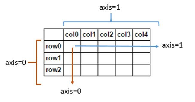
In this context, if you see or hear the term "axis", assume the speaker is talking about the layout of your dataframe as opposed to the dimensionality of your features. We will go into more detail about this as it comes up.
View Column DataTypes
When you load up a dataframe, it's always a good idea to see what data type Pandas assigned each column:
>>> df.dtypesrecency int64history_segment objecthistory float64mens int64womens int64zip_code objectnewbie int64channel objectsegment objectvisit int64conversion int64spend float64DM_category int64dtype: object
Pandas will check your dataset and then on a per-column basis will decide if it's a numeric-type: int32, float32, float64. date-type: datetime64, timedelta[ns]. Or other object-type: object (string), category. If Pandas incorrectly assigns a type to a column, you can convert it, and we'll discuss that later on.
Slicin' and Dicin', Part One
NOTE: To follow the instruction below, make sure you download the zip file found in the Setting Up Your Lab Environment section.
In this lesson, you'll learn how to intuitively select of a subset of data out of your dataframes or series, an operation known as indexing. More than half of the top-voted StackOverflow questions on Pandas revolve around this single topic! This shows you how important and potentially confusing indexing can be. Spend adequate time working through this chapter and playing around with the accompanying dataset.
Learning to properly indexing is like learning the ABC's, so if you have a gap in your indexing knowledge, it'll be hard to complete future tasks. But if you're able to master this, you'll have mastered the building blocks of all future material. To get you accustomed to indexing, first use the .read_csv() method you just learned about to load up the direct_marketing.csv file in your course /Module2/Datasets/ directory:
>>> df = pd.read_csv('Datasets/direct_marketing.csv')
>>> df

       recency   history_segment  history  mens  womens   zip_code  newbie
0           10    2) $100 - $200   142.44     1       0  Surburban       0
1            6    3) $200 - $350   329.08     1       1      Rural       1
2            7    2) $100 - $200   180.65     0       1  Surburban       1
3            9    5) $500 - $750   675.83     1       0      Rural       1
4            2      1) $0 - $100    45.34     1       0      Urban       0
5            6    2) $100 - $200   134.83     0       1  Surburban       0
Column Indexing
A dataframe is essentially one or more series which have been 'stitched' together into a new data type. Pandas exposes many equivalent methods for slicing out those underlying series. You can slice by location, the way you would normally index into a regular Python list. You can slice by label, the way you would normally index into a Python dictionary. And like NumPy arrays, you can also index by boolean masks:
>>> df.recency
>>> df['recency']
>>> df[['recency']]
>>> df.loc[:, 'recency']
>>> df.loc[:, ['recency']]
>>> df.iloc[:, 0]
>>> df.iloc[:, [0]]
>>> df.ix[:, 0]
Why does Pandas have so many different data access methods? The answer is because there are slight differences between them. The first difference you'll notice from the list above is that in some of the commands, you specify the name of the column or series you want to slice: recency. By using the column name in the code, it's very easy to discern what is being pulled, and you don't have to worry about the order of the columns. Doing this lookup of first matching the column name before slicing the column index is marginally slower than directly accessing the column by index.
Once you're ready to move to a production environment, Pandas documentation recommends you use either .loc[], .iloc[], or .ix[] data access methods, which are more optimized. The .loc[] method selects by column label, .iloc[] selects by column index, and .ix[] can be used whenever you want to use a hybrid approach of either. All code in this course will use either the df.recency or df[['recency', ...]] data-access syntax styles for maximum clarity.
Another difference you'll notice is that some of the methods take in a list of parameters, e.g.: df[['recency']], df.loc[:, ['recency']], and df.iloc[:, [0]]. By passing in a list of parameters, you can select more than one column to slice. Please be aware that if you use this syntax, even if you only specify a single column, the data type that you'll get back is a dataframe as opposed to a series. This will be useful for you to know once you start machine learning, so be sure to take down that note.
#
# Produces a series object:
>>> df.recency
>>> df['recency']
>>> df.loc[:, 'recency']
>>> df.iloc[:, 0]
>>> df.ix[:, 0]

0        10
1         6
2         7
3         9
4         2
5         6
Name: recency, dtype: int64

#
# Produces a dataframe object:
>>> df[['recency']]
>>> df.loc[:, ['recency']]
>>> df.iloc[:, [0]]

       recency
0           10
1            6
2            7
3            9
4            2
5            6

[64000 rows x 1 columns]
Row Indexing
You can use any of the .loc[], .iloc[], or .ix[] methods to do selection by row, noting that the expected order is [row_indexer, column_indexer]:
>>> df[0:2]
>>> df.iloc[0:2, :]

   recency history_segment  history  mens  womens   zip_code  newbie channel
0       10  2) $100 - $200   142.44     1       0  Surburban       0   Phone
1        6  3) $200 - $350   329.08     1       1      Rural       1     Web
The last important difference is that .loc[] and .ix[] are inclusive of the range of values selected, where .iloc[] is non-inclusive. In that sense, df.loc[0:1, :] would select the first two rows, but only the first row would be returned using df.iloc[0:1, :].
Slicin' and Dicin', Part Two
Boolean Indexing
Your dataframes and series can also be indexed with a boolean operation—a dataframe or series with the same dimensions as the one you are selecting from, but with every value either being set to True or False. You can create a new boolean series either by manually specifying the values, or by using a conditional:
>>> df.recency < 7

0        False
1         True
2        False
3        False
4         True
5         True

Name: recency, dtype: bool
To index with your boolean series, simply feed it back into your regular series with using the [] bracket-selection syntax. The result is a new series that once again has the same dimensions, however only values corresponding to True values in the boolean series get returned:
>>> df[ df.recency < 7 ]

       recency   history_segment  history  mens  womens   zip_code  newbie
1            6    3) $200 - $350   329.08     1       1      Rural       1
4            2      1) $0 - $100    45.34     1       0      Urban       0
5            6    2) $100 - $200   134.83     0       1  Surburban       0
If you need even finer grain control of what gets selected, you can further combine multiple boolean indexing conditionals together using the bit-wise logical operators | and &:
>>> df[ (df.recency < 7) & (df.newbie == 0) ]

       recency history_segment  history  mens  womens   zip_code  newbie
4            2    1) $0 - $100    45.34     1       0      Urban       0
5            6  2) $100 - $200   134.83     0       1  Surburban       0
This is a bit counter-intuitive, as most people initially assume Pandas would support the regular, Python boolean operators or and and. The reason regular Python boolean operators cannot be used to combine Pandas boolean conditionals is because doing so causes ambiguity. There are two ways the following incorrect statement can be interpreted (df.recency<7) or (df.newbie==0):
If the evaluation the statement (df.recency<7) or the evaluation the statement (df.newbie==0) results in anything besides the False, then select all records in the dataset.
Select all columns belonging to rows in the dataset where either of the following statements are true: (df.recency<7) or (df.newbie==0).
Option 2 is the desired functionality, but to avoid this ambiguity entirely, Pandas overloads bit-wise operators on its dataframe and series objects. Be sure to encapsulate each conditional in parenthesis to make this work.
Writing to a Slice
Something handy that you can do with a dataframe or series is write into a slice:
>>> df[df.recency < 7] = -100
>>> df

       recency   history_segment  history  mens  womens   zip_code  newbie
0           10    2) $100 - $200   142.44     1       0  Surburban       0
1         -100              -100  -100.00  -100    -100       -100    -100
2            7    2) $100 - $200   180.65     0       1  Surburban       1
3            9    5) $500 - $750   675.83     1       0      Rural       1
4         -100              -100  -100.00  -100    -100       -100    -100
5         -100              -100  -100.00  -100    -100       -100    -100
Take precaution while doing this, as you may encounter issues with non-homogeneous dataframes. It is far safer, and generally makes more sense, to do this sort of operation on a per column basis rather than across your entire dataframe. In the above example, -100 is rendered as an integer in the recency column, a string in the history_segment column, and a float in the history column.
Feature Representation
Your features need be represented as quantitative (preferably numeric) attributes of the thing you're sampling. They can be real world values, such as the readings from a sensor, and other discernible, physical properties. Alternatively, your features can also be calculated derivatives, such as the presence of certain edges and curves in an image, or lack thereof.
If your data comes to you in a nicely formed, numeric, tabular format, then that's one less thing for you to worry about. But there is no guarantee that will be the case, and you will often encounter data in textual or other unstructured forms. Luckily, there are a few techniques that when applied, clean up these scenarios.
Textual Categorical-Features
If you have a categorical feature, the way to represent it in your dataset depends on if it's ordinal or nominal. For ordinal features, map the order as increasing integers in a single numeric feature. Any entries not found in your designated categories list will be mapped to -1:
>>> ordered_satisfaction = ['Very Unhappy', 'Unhappy', 'Neutral', 'Happy', 'Very Happy']
>>> df = pd.DataFrame({'satisfaction':['Mad', 'Happy', 'Unhappy', 'Neutral']})
>>> df.satisfaction = df.satisfaction.astype("category",
  ordered=True,
  categories=ordered_satisfaction
).cat.codes

>>> df
   satisfaction
0            -1
1             3
2             1
3             2
On the other hand, if your feature is nominal (and thus there is no obvious numeric ordering), then you have two options. The first is you can encoded it similar as you did above. This would be a fast-and-dirty approach. While you're just getting accustomed to your dataset and taking it for its first run through your data analysis pipeline, this method might be best:
>>> df = pd.DataFrame({'vertebrates':[
...  'Bird',
...  'Bird',
...  'Mammal',
...  'Fish',
...  'Amphibian',
...  'Reptile',
...  'Mammal',
... ]})

# Method 1)
>>> df['vertebrates'] = df.vertebrates.astype("category").cat.codes

>>> df
  vertebrates  vertebrates
0        Bird            1
1        Bird            1
2      Mammal            3
3        Fish            2
4   Amphibian            0
5     Reptile            4
6      Mammal            3
Notice how this time, ordered=True was not passed in, nor was a specific ordering listed. Because of this, Pandas encodes your nominal entries in alphabetical order. This approach is fine for getting your feet wet, but the issue it has is that it still introduces an ordering to a categorical list of items that inherently has none. This may or may not cause problems for you in the future. If you aren't getting the results you hoped for, or even if you are getting the results you desired but would like to further increase the result accuracy, then a more precise encoding approach would be to separate the distinct values out into individual boolean features:
# Method 2)
>>> df = pd.get_dummies(df,columns=['vertebrates'])

>>> df
   vertebrates_Amphibian  vertebrates_Bird  vertebrates_Fish  \
0                    0.0               1.0               0.0
1                    0.0               1.0               0.0
2                    0.0               0.0               0.0
3                    0.0               0.0               1.0
4                    1.0               0.0               0.0
5                    0.0               0.0               0.0
6                    0.0               0.0               0.0

   vertebrates_Mammal  vertebrates_Reptile
0                 0.0                  0.0
1                 0.0                  0.0
2                 1.0                  0.0
3                 0.0                  0.0
4                 0.0                  0.0
5                 0.0                  1.0
6                 1.0                  0.0
These newly created features are called boolean features because the only values they can contain are either 0 for non-inclusion, or 1 for inclusion. Pandas .get_dummies() method allows you to completely replace a single, nominal feature with multiple boolean indicator features. This method is quite powerful and has many configurable options, including the ability to return a SparseDataFrame, and other prefixing options. It's benefit is that no erroneous ordering is introduced into your dataset.
Pure Textual Features
If you are trying to "featurize" a body of text such as a webpage, a tweet, a passage from a newspaper, an entire book, or a PDF document, creating a corpus of words and counting their frequency is an extremely powerful encoding tool. This is also known as the Bag of Words model, implemented with the CountVectorizer() method in SciKit-Learn. Even though the grammar of your sentences and their word-order are complete discarded, this model has accomplished some pretty amazing things, such as correctly identifying J.K. Rowling's writing from a blind line up of authors.
>>> from sklearn.feature_extraction.text import CountVectorizer

>>> corpus = [
...  "Authman ran faster than Harry because he is an athlete.",
...  "Authman and Harry ran faster and faster.",
... ]

>>> bow = CountVectorizer()
>>> X = bow.fit_transform(corpus) # Sparse Matrix

>>> bow.get_feature_names()
['an', 'and', 'athlete', 'authman', 'because', 'faster', 'harry', 'he', 'is', 'ran', 'than']

>>> X.toarray()
[[1 0 1 1 1 1 1 1 1 1 1]
 [0 2 0 1 0 2 1 0 0 1 0]]
Some new points of interest. X is not the regular [n_samples, n_features] dataframe you are familiar with. Rather, it is a SciPy compressed, sparse, row matrix. SciPy is a library of mathematical algorithms and convenience functions that further extend NumPy. The reason X is now a sparse matrix instead of a classical dataframe is because even with this small example of two sentences, 11 features got created. The average English speaker knows around 8000 unique words. If each sentence were an 8000-sized vector sample in your dataframe, consisting mostly of 0's, it would be a poor use of memory.
To avoid this, SciPy implements their sparse matrices like Python implements its dictionaries: only the keys that have a value get stored, and everything else is assumed to be empty. You can always convert it to a regular Python list by using the .toarray() method, but this converts it to a dense array, which might not be desirable due to memory reasons. To use your compressed, spare, row matrix in Pandas, you're going to want to convert it to a Pandas SparseDataFrame. More notes on that in the Dive Deeper section.
The bag of words model has other configurable parameters, such as considering the order of words. In such implementations, pairs or tuples of successive words are used to build the corpus instead of individual words:
>>> bow.get_feature_names()
['authman ran', 'ran faster', 'faster than', 'than harry', 'harry because', 'because he', 'he is', 'is an', 'an athlete', 'authman and', 'and harry', 'harry ran', 'faster and', 'and faster']
Another parameter is to have it use frequencies ant not counts. This is useful when you have documents of different lengths, so to allow direct comparisons even though the raw counts for the longer document would of course be higher. Dive deeper into the feature extraction section of SciKit-Learn's documentation to learn more about how you can best represent your textual features!
Graphical Features
In addition to text and natural language processing, bag of words has successfully been applied to images by categorizing a collection of regions and describing only their appearance, ignoring any spatial structure. However this is not the typical approach used to represent images as features, and requires you come up with methods of categorizing image regions. More often used methods include:
Split the image into a grid of smaller areas, and attempt feature extraction at each locality. Return a combined array of all discovered. features
Use variable-length gradients and other transformations as the features, such as regions of high / low luminosity, histogram counts for horizontal and vertical black pixels, stroke and edge detection, etc.
Resize the picture to a fixed size, convert it to grayscale, then encode every pixel as an element in a uni-dimensional feature array.
Let's explore how you might go about using the third method with code:
# Uses the Image module (PIL)
from scipy import misc

# Load the image up
img = misc.imread('image.png')

# Is the image too big? Resample it down by an order of magnitude
img = img[::2, ::2]

# Scale colors from (0-255) to (0-1), then reshape to 1D array per pixel, e.g. grayscale
# If you had color images and wanted to preserve all color channels, use .reshape(-1,3)
X = (img / 255.0).reshape(-1)

# To-Do: Machine Learning with X!
#
If you're wondering what the :: is doing, that is called extended slicing. Notice the .reshape(-1) line. This tells Pandas to take your 2D image and flatten it into a 1D array. This is an all purpose method you can use to change the shape of your dataframes, so long as you maintain the number of elements. For example reshaping a [6, 6] to [36, 1] or [3, 12], etc. Another method called .ravel() will do the same thing as .reshape(-1), that is unravel a multi-dimensional NDArray into a one dimensional one. The reason why its important to reshape your 2D array images into one dimensional ones is because each image will represent a single sample, and SKLearn expects your dataframe to be shapes [num_samples, num_features].
Since each image is treated as a single sample, your datasets likely need to have many image samples within them. You can create a dataset of images by simply adding them to a regular Python list and then converting the whole thing in one shot:
# Uses the Image module (PIL)
from scipy import misc

# Load the image up
dset = []
for fname in files:
  img = misc.imread(fname)
  dset.append(  (img[::2, ::2] / 255.0).reshape(-1)  )

dset = pd.DataFrame( dset )
Audio Features
Audio can be encoded with similar methods as graphical features, with the caveat that your 'audio-image' is already a one-dimensional waveform data type instead of a two-dimensional array of pixels. Rather than looking for graphical gradients, you would look for auditory ones, such as the length of sounds, power and noise ratios, and histogram counts after applying filters.
import scipy.io.wavfile as wavfile

sample_rate, audio_data = wavfile.read('sound.wav')
print audio_data

# To-Do: Machine Learning with audio_data!
#
